Regardless of the recent advancements in ultrasonic flaw detectors, ultrasonic software and, phased array ultrasonic testing technology, the best practice for ultrasonic shear wave inspectors remains the ability to plot a weld profile and the interaction of ultrasonic soundwaves at refracted angles. Today, some of the advanced ultrasonic instruments produce a weld overlay on the screen. Others identify the 1st, 2nd and 3rd legs of the soundwave by color.
For many years, manual plotting has been used to develop a successful understanding and interpretation of the received signals from either the geometric features of a weld or from a weld discontinuity. Clear plotting during shear wave ultrasonic testing (UT) will certainly prove beneficial to those developing an initial understanding, especially for those taking practical exams in UT shear wave weld inspection, such as the American Petroleum Institute Qualification of Ultrasonic Testing Examiners Program Detection and Sizing Test.
The discontinuity depth is an important piece of information that a level II UT technician should determine during the ultrasonic inspection of welds, based on the receiving signals from a weld discontinuity. In UT of CJP welds in a butt joint configuration, discontinuity depth, D, is defined as the distance from the discontinuity to the transducer side of the base metal. The capability of the UT technique to provide this piece of information is one of the greatest advantages of the UT method compared to typical radiographic testing methods (Figure 2a).
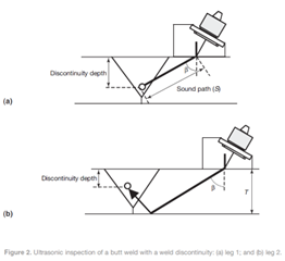
If the receiving signal of a weld discontinuity is reflected directly by the discontinuity, it is usually referred to as leg 1 (Figure 2a), and if the receiving signal comes after one reflection from the other side of the base metal, it is called leg 2 (Figure 2b). Both leg 1 and leg 2 can be calculated easily or can be determined experimentally and on the UT flaw detector screen, which helps to indicate whether the receiving signals come from the first leg or second leg. Simple geometric formulas are used to calculate the discontinuity depth based on the refracted angle (), sound path distance (S) and thickness of the base metal (T).
- D_leg1=(cosβ)S D_leg2=2T-(cosβ)S
Usually, the second formula is somewhat more difficult for UT technicians to understand and to remember (trainees usually ask how the term 2T appears in the second formula). To illustrate this second case, plotting and a simple visual aid can be helpful.
Procedure
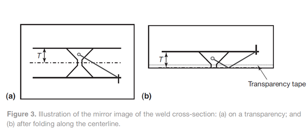
Take a piece of transparent film (used on overhead projectors) and draw to scale a mirror image of the weld cross-section on it. On the drawing show an imaginary weld discontinuity and the ultrasonic beam (Figure 3a). To simplify the process at this stage, only draw the refracted beam from one side of the weld (first leg). Use colored markers to identify the sound paths. Cut the transparency film exactly along the centerline of the weld and then tape these pieces together using transparent tape, edge to edge, leaving a small gap between them. Now, if the drawing is folded along the taped section (Figure 3b), then an image will appear exactly as shown in Figure 2b for the leg 2 case.
Due to the symmetry in the mirror image and the geometry that applies to the ultrasonic beam (Figure 3b), the total sound path distance of the ultrasonic beam in the leg 2 case as reflected from the other surface is indeed the same as the straight line in Figure 3a.
Calculations
If the transparency is unfolded (Figure 4), the distance, D, is simply:
(2) D=2T-h
where h can be found exactly as in the leg 1 case.
(3) h=(cosβ)S
If h is substituted in Equation 1, we get the relationship that we were looking for.
(4) h=(cosβ)S
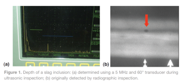
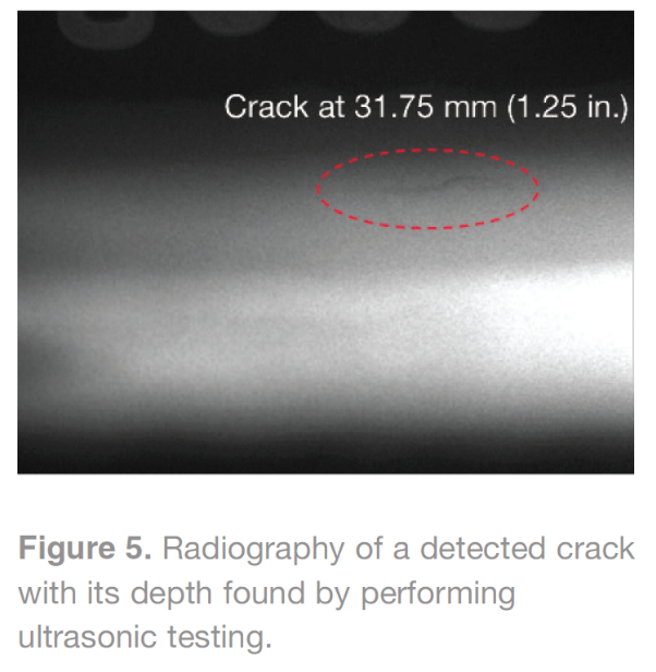
Figure 5 shows an example, where the formula for leg 2 was used during the UT inspection to calculate the depth of a solidification crack in a 50.8 mm (2 in.) weld, originally detected during radiography inspection. The sound path (S) of the receiving signal was 140 mm (5.5 in.) using a 5 MHz transducer with 60° refracted angle. Applying the leg 2 calculation produces the following.
(5) D_leg2=2T-(cosβ)S, D_leg2=2×2-(cos60°)5.5,D_leg2=1.25in.
Normally, the wave propagation within any given specimen is more complex due to its beam spreading, the interaction with different boundaries, and its mode conversion. However, this simple demonstration helps UT technicians recall the formula during their weld inspection, and provides a better understanding and interpretation of reflected signals.